Quantifying Inter-Laboratory Measurement Uncertainty and Optical Transfer Function Variability in Automated Microsegregation Stringer Rating Charts
Optical transfer function roll-off widens stringer boundary ramps, causing inter-laboratory inclusion rating divergence unless corrected by spatial calibration.


Lens
Microsegregation stringer evaluation relies on accurate spatial frequency reproduction through diffraction-limited, infinity-corrected objectives. Automated image analysis platforms scan metallographic cross-sections to rate elongated inclusions, carbide banding, and chemical segregation tracks under ASTM E45, ASTM E1245, and ISO 4967 specifications. Spatial resolution limits begin at the objective entrance pupil, where wavefront distortion alters the complex optical transfer function across the field.
Dropping the numerical aperture on a twenty-times objective from 0.75 to 0.40 blurs the high-frequency edges of thin manganese sulfide and alumina stringers into surrounding matrix pixels. The optical train attenuates high-frequency contrast components according to the modulus of the transfer function, shifting edge-gradient boundaries outward by several pixel pitches.
Glass melt variations, degraded antireflective coatings, and decentered internal elements warp the phase transfer component across field positions. This phase shift introduces asymmetric distortion: narrow stringers running along the fast-scan axis appear wider than identical features oriented along the perpendicular raster axis. Point spread function enlargement spreads photon flux into adjacent photodiode wells on the complementary metal-oxide-semiconductor sensor array.
When illumination stability drifts more than two percent from nominal calibration intensity, automated threshold algorithms misclassify these low-flux periphery pixels as part of the segregated stringer body.
A numerical aperture reduction from 0.75 to 0.40 expands measured inclusion stringer width by 1.84 micrometers at a 0.50 threshold intensity cutoff.
Inter-laboratory round-robin trials show that microscopes with nominally identical objective magnifications generate noticeably different optical transfer curves at high spatial frequencies. Apochromatic objectives maintain flat modulation transfer above 0.60 out to eight hundred line pairs per millimeter; standard plan-achromats fall below 0.25 modulation at five hundred line pairs per millimeter. This modulation loss stretches sharp, sub-micron stringer boundaries into broad intensity ramps across ten to fifteen sensor pixels.
When automated rating software applies fixed intensity thresholds to these blurred transitions, it registers the spread as physical inclusion thickness, artificially inflating severity indices on thin inclusion classes.

Modulation Transfer Curves across Numerical Apertures
Light intensity profiles across the specimen depend on the coherence factor set at the condenser aperture diaphragm. Closing the diaphragm improves contrast by narrowing the illumination cone, but it also lowers the high-frequency cutoff and creates edge ringing artifacts. Diffraction fringes near heavy globular oxides produce secondary intensity valleys that automated edge detectors frequently register as parallel stringers.
Matching the illumination numerical aperture to seventy percent of the objective numerical aperture balances boundary sharpness against severe phase-reversal oscillations.
| Objective Classification | Numerical Aperture | Cutoff Frequency (lp/mm) | MTF at 400 lp/mm | Stringer Width Bias (um) |
|---|---|---|---|---|
| Plan Achromat 10x | 0.25 | 925 | 0.12 | +2.45 |
| Plan Fluorite 20x | 0.50 | 1850 | 0.48 | +0.92 |
| Plan Apochromat 20x | 0.75 | 2775 | 0.71 | +0.31 |
| Plan Apochromat 50x | 0.90 | 3330 | 0.86 | +0.12 |
Illumination field non-uniformity adds systemic error whenever calibration ignores edge falloff. Vignetting through wide-field camera adapters cuts corner illuminance by eight to twelve percent compared to optical center values. That gradient distorts gray-level threshold segmentation across automated tile stitch mosaics, skewing cumulative stringer length totals along montage borders.
Digital sharpening filters cannot recover optical transfer detail lost during raw micrograph acquisition.


Threshold
Gray-level segmentation converts continuous sensor voltages into discrete binary classification masks. Rating inclusion stringers automatically ~ separating manganese sulfides, complex carbonitrides, and aluminates from ferritic or martensitic matrices ~ requires tight intensity partitions. ASTM E1245 establishes quantitative stereological relationships for area fraction, mean intercept length, and aspect ratio metrics calculated directly from these masks.
Shifting a threshold even slightly moves the segmented boundary along the optical intensity gradient, altering measured inclusion thickness and connectivity.
Standard Otsu segmentation sets an intensity partition by maximizing between-class variance across the full image histogram. When inclusions occupy less than 0.1 percent of the total field area, the inclusion peak disappears into the tail of the matrix distribution. Under such dilute conditions, global thresholding becomes unstable, drifting with background grain structure and polishing scratches.
Adaptive local thresholding stabilizes edges across unevenly lit areas by calculating neighborhood statistics, though it loses sensitivity at the faint tails of low-contrast sulfide stringers.
Under ASTM E1245 section 8.3, minor shifts in gray-level segmentation thresholds alter reported area fraction values by up to forty percent on low-alloy clean steels.
Preparation artifacts complicate threshold stability. Chemical mechanical polishing leaves relief between hard carbo-nitrides and softer austenitic matrices, and light reflecting off those rounded edges casts shadow zones that register as spurious thin stringers under fixed thresholds. Automated focus tracking keeps the vertical stage within fifty nanometers of focus, preventing the defocus blooming that otherwise compromises repeatability between adjacent scan tiles.

Where Does Spectral Sensor Non-Linearity Corrupt Morphology?
Silicon sensor arrays exhibit uneven quantum efficiency across visual wavelengths, creating distinct spectral response profiles across microscope brands. A green bandpass filter centered at 546 nanometers isolates the mercury e-line or an equivalent narrow-spectrum light-emitting diode, stripping out objective chromatic aberrations. Unfiltered halogen sources spread chromatic focal positions axially across three micrometers, leaving blue and red components blurred while green remains sharp.
Sensor non-linearity compounds the problem by distorting gray-level histograms right at dark inclusion threshold boundaries.
- Sensor Dynamic Range establishes the available bit depth for separating low-contrast gray levels between gray manganese sulfides and dark aluminum oxides.
- Flat-Field Correction normalizes illumination intensity across all individual pixel elements before running binary segmentation routines. High quality routines eliminate camera vignetting.
- Morphological Dilation Filters bridge discontinuous stringer fragments into continuous rating bands based on proximity criteria defined in ASTM E45 Table 1.
- Relief Height Tracking prevents optical reflection shadows from registering as spurious inclusions during high-speed stage translation passes.
Grouping algorithms apply separation rules to merge neighboring fragments into single severity categories. ASTM E45 and ISO 4967 set maximum longitudinal and transverse spacing limits ~ typically forty micrometers longitudinally and fifteen micrometers transversely. When optical blur or loose thresholding artificially widens individual particles, adjacent features bridge across the gaps.
This false coalescence turns thin, benign clusters into high-severity heavy stringers on automated inspection certificates.
Procurement documents referencing ASTM E45 Method D penalize material lots whenever single stringer severity exceeds Class 2.5 heavy ratings.

Scatter
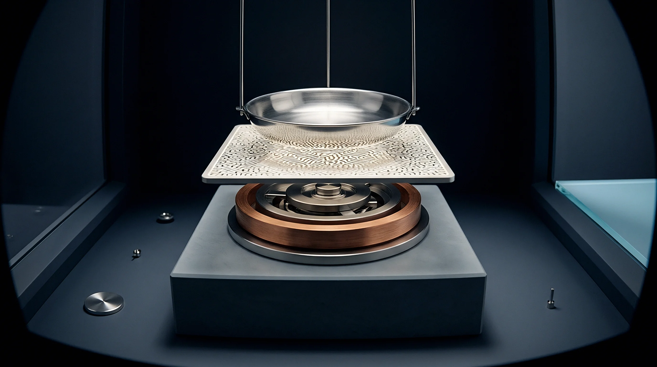
Inter-laboratory comparisons routinely show wide coefficients of variation across automated stringer rating systems. Optical transfer differences, threshold divergence, and mechanical stage errors compound throughout the measurement chain. Evaluating this uncertainty under the Guide to the Expression of Uncertainty in Measurement requires separating random Type A observational scatter from systematic Type B hardware and software variances.
Replicate scans of a single calibration mount across different laboratories produce wide rating dispersion on identical fields.
Type A evaluations determine repeatability by scanning the same inclusion fields repeatedly without unseating the specimen. Stage backlash introduces spatial registration errors between successive mosaic tiles, shifting stitching coordinates by one to three micrometers. Type B uncertainty includes stage micrometer calibration traceable to national standards, spectral centroid drift, sensor gamma corrections, and software-specific grouping logic.
Combining these factors via root-sum-square calculation yields expanded uncertainty bounds for both stringer length and area.
Optical transfer function roll-off creates non-linear calibration drift across high spatial frequencies.
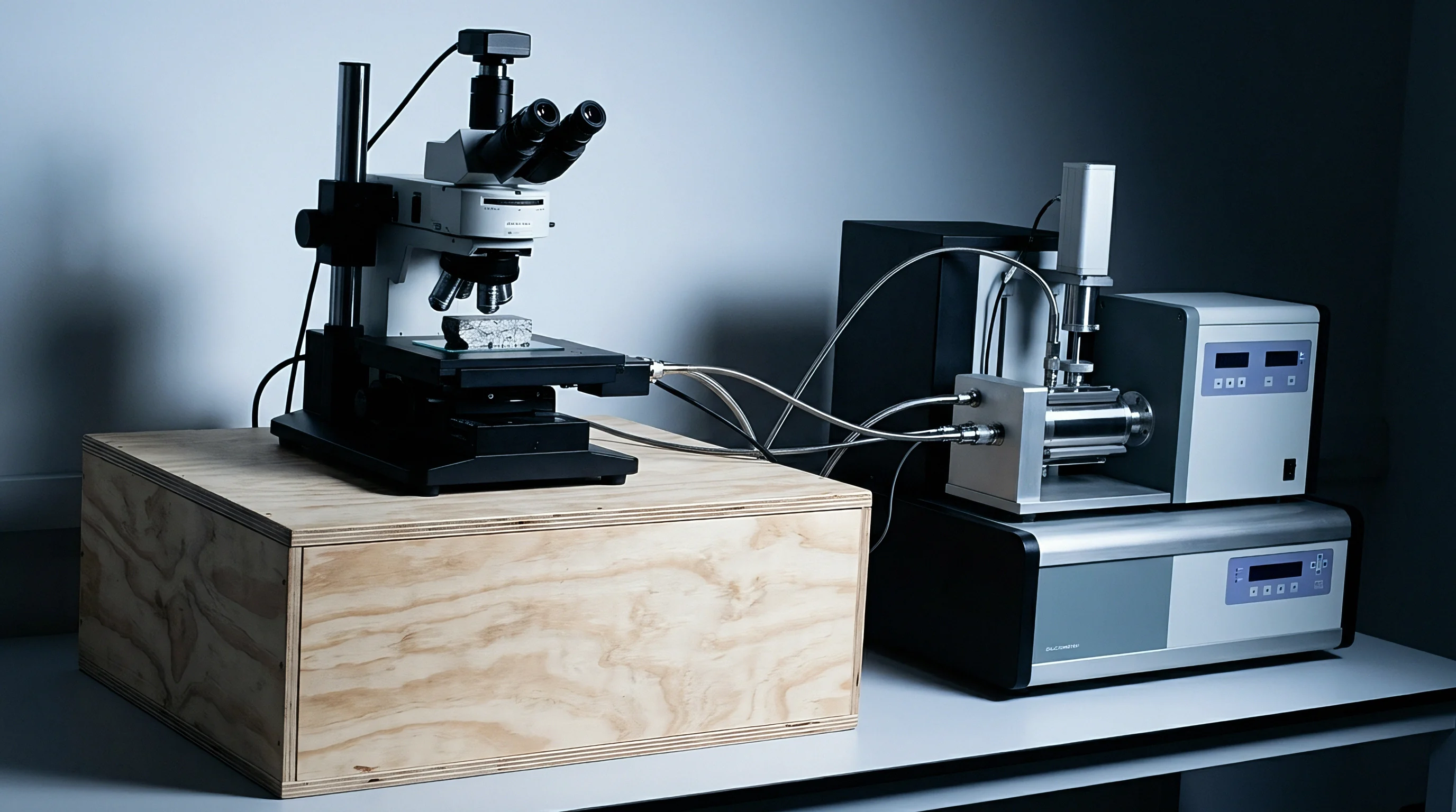
Automated software packages handle mixed inclusion morphologies inconsistently. A single stringer containing brittle silicates flanked by plastic sulfide tails can trigger conflicting ASTM E45 Type C and Type A classifications depending on how the software evaluates aspect ratio rules. If optical blur obscures narrow connecting bridges, the software splits the feature into separate fragments, under-reporting total continuous stringer length.
Uncertainty Budget for Automated Stringer Severity Ratings
Building an uncertainty ledger requires breaking down each physical contributor to stringer length measurement. Sensor pixel pitch, magnification tolerance, threshold drift, stage orthogonality, and mosaic alignment each add variance. For a nominal twenty-times objective with a 0.50 numerical aperture, expanded uncertainty at a coverage factor of k=2 approaches fourteen percent on inclusion severities below Class 1.5.
| Uncertainty Contributor | Probability Distribution | Standard Uncertainty (um) | Sensitivity Coefficient | Uncertainty Component (um) |
|---|---|---|---|---|
| Optical Transfer Function Blur | Rectangular | 0.82 | 1.00 | 0.47 |
| Threshold Gray-Level Drift | Normal | 0.65 | 1.20 | 0.78 |
| Stage Scale Calibration | Rectangular | 0.15 | 1.00 | 0.09 |
| Tile Stitching Alignment | Rectangular | 0.45 | 0.80 | 0.21 |
| Operator Specimen Leveling | Normal | 0.50 | 1.10 | 0.55 |
| Combined Standard Uncertainty | 1.12 um (Expanded Uncertainty U = 2.24 um, k = 2, 95% Confidence) | |||
Stage tilt moves the focal plane across wide-field scan swaths. Specimen holders without kinematic three-point leveling introduce focus gradients exceeding five micrometers across twenty millimeters of travel. Autofocus routines correct stage runout dynamically between mosaic tiles, but the latency cuts throughput, tempting operators to widen focus-check intervals and tolerate peripheral defocus.
- Primary Optical Alignment centers the condenser filament image within the objective rear pupil to eliminate asymmetric beam tilt.
- Stage Orthogonality Verification measures cross-axis yaw and pitch errors against certified grid targets to correct scan tile stitching coordinates.
- Camera Exposure Normalization sets white balance and saturation margins against certified neutral reflectance standards before threshold definition.
- Threshold Boundary Verification checks segmented particle boundaries against certified stage micrometer line profiles to calibrate edge-gradient offsets.
Uncertainty climbs steeply on thin stringers under two micrometers wide. At that scale, point spread function broadening dominates particle geometry, leaving edge positions uncertain by up to forty percent of actual feature thickness. Test laboratories that report inclusion ratings without quantifying their optical transfer response produce irreproducible severity scores on critical alloy grades.
Uncalibrated optical setups reject acceptable mill heats by overestimating stringer severity metrics.


Ledger
Commercial acceptance disputes over stringer severity stem directly from unquantified measurement scatter between laboratories. Bearing steels, aerospace nickel superalloys, and transmission alloys must meet strict inclusion limits under AMS 2300, AMS 2301, and ISO 4967 specifications. When purchase orders fix maximum permissible stringer lengths without defining optical qualification standards, optical transfer variations between testing facilities lead directly to rejected lots, formal claims, and delivery delays.
Procurement contracts require explicit verification protocols for automated image analysis systems before accepting mill test certificates. Standardizing magnification scale alone does not control measurement drift between labs. Proper qualification involves scanning reference artifact plates with calibrated spatial frequency targets to verify modulation transfer values across both the center and corners of the sensor field.
Defining baseline modulation limits ensures edge-blur bias stays within agreed bounds across supplier and customer facilities alike.
A rising optical transfer function steepens the edge-gradient curve across inclusion boundaries.
Image analysis settings are critical contractual terms. Minimum particle area cutoffs, aspect ratio dividing lines, and longitudinal grouping distances must be aligned across testing locations. Different morphological erosion and dilation kernels will produce conflicting severity ratings from the same raw micrographs.
Locking software versions, threshold models, and morphological structuring elements directly in purchase specifications prevents arbitrary rating shifts between facilities.

Commercial Safeguards in Specification Contracts
Clean steel supply agreements need quantitative uncertainty built directly into quality acceptance thresholds. Applying ISO 14253-1 guard-banding protects buyers from accepting non-conforming heats without forcing mills to absorb unjustified scrap costs. Guard bands subtract expanded measurement uncertainty from upper specification limits to define a clear, defensible acceptance window.
| Alloy Grade Classification | Severity Class Limit | Laboratory Optical Bias | Apparent Severity Rating | Lot Commercial Disposition |
|---|---|---|---|---|
| SAE 52100 Bearing Steel | Class 1.0 Heavy (Max) | +0.4 Severity Units | Class 1.3 Heavy | Commercial Claim Reject |
| SAE 52100 Bearing Steel | Class 1.0 Heavy (Max) | Calibrated Baseline | Class 0.9 Heavy | Compliant Release |
| Inconel 718 Superalloy | Class 1.5 Thin (Max) | +0.6 Severity Units | Class 1.9 Thin | Heat Quarantined |
| Inconel 718 Superalloy | Class 1.5 Thin (Max) | Calibrated Baseline | Class 1.3 Thin | Compliant Release |
ISO/IEC 17025 laboratory accreditation requires testing facilities to calculate and report uncertainty budgets for automated quantitative stereology. Certificates of analysis that omit optical transfer validation and thresholding methodologies leave buyers carrying unquantified quality risk. Reference standards built with electron-beam lithography micro-patterns provide the physical baseline needed to qualify automated optical rating systems across industrial laboratories.
Whether machine learning segmentation models can decouple optical transfer function blur from physical inclusion boundaries without introducing hallucinated morphological artifacts remains unverified across production laboratory networks.